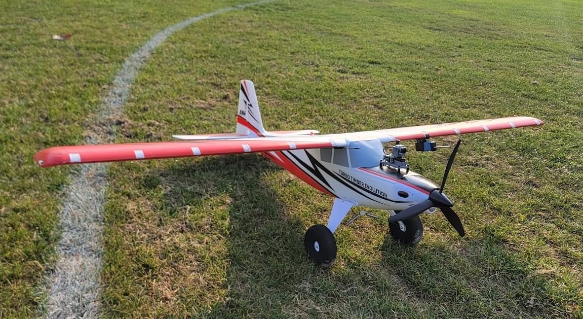
A multicopter is unstable without active control. If the autopilot stops correcting attitude for even a fraction of a second, the vehicle starts to tumble. Flight control is therefore one of the clearest examples of a hard real-time embedded system. A small processor has to sample inertial sensors, estimate the vehicle’s state, compute control outputs and drive the motors, over and over, with tightly bounded latency and jitter. Telemetry, logging, navigation and payload handling run on the same processor at the same time.
This article explains how flight control software is structured around timing, using the two dominant open-source autopilots, PX4 and ArduPilot, as concrete examples. It also covers how control theory sets the timing requirements and what assurance standards such as DO-178C expect when an autopilot has to be certified.
Key takeaways
- Flight control uses cascaded loops. The fast inner angular-rate loop has the tightest timing, and outer attitude, velocity and position loops run progressively slower.
- What matters most is sample-to-actuation latency and its jitter. Every millisecond of delay adds phase lag and erodes stability margins.
- PX4 runs on the NuttX RTOS and organizes modules around the uORB publish/subscribe bus and prioritized work queues, with the rate controller driven by new gyro data.
- ArduPilot uses a main-loop scheduler: a fast loop runs every tick, and a task table assigns each task a rate and a time budget.
- Certified avionics under DO-178C must show worst-case timing evidence, and multicore processors bring additional interference guidance.
The cascaded control loop hierarchy
Almost every multirotor and fixed-wing autopilot uses a cascade of feedback loops. Each outer loop produces the setpoint for the loop inside it:
- Position / navigation turns waypoints or pilot commands into velocity setpoints.
- Velocity turns velocity error into desired acceleration, which becomes desired attitude and thrust.
- Attitude turns attitude error into desired angular rates.
- Angular rate turns rate error, measured directly by the gyroscope, into torque commands. These go through a mixer to individual motor outputs.
A cascade works well when each inner loop is substantially faster than the loop around it. The rate loop is therefore the timing-critical core. A state estimator, usually an extended Kalman filter (EKF) fusing IMU, GNSS, magnetometer, barometer and other sensors, supplies the attitude, velocity and position estimates the outer loops need.
| Function | Typical order of magnitude | Timing sensitivity |
|---|---|---|
| IMU sampling (gyro/accel) | Often kHz range, buffered in sensor FIFOs | Sample timing and timestamp accuracy |
| Angular-rate control loop | Hundreds of Hz to kHz | Very high: latency and jitter directly affect stability |
| Attitude control loop | Same as or lower than rate loop | High |
| State estimation (EKF) | Tens to hundreds of Hz, depending on design | High: stale estimates degrade outer loops |
| Velocity / position control | Tens of Hz to around a hundred Hz | Medium |
| Navigation, mission logic | Low tens of Hz or less | Low to medium |
| Telemetry, logging | Variable, best effort | Low, but must not starve or block control |
The ranges are deliberately broad. Actual rates depend on the airframe, the autopilot, the board and the configuration. Small racing quads often run their inner loops much faster than large, slow fixed-wing aircraft do.
Why latency and jitter matter: a control view
From a control-theory point of view, a pure time delay τ adds phase lag that grows with frequency: φ = −360° · f · τ. At a loop crossover frequency of 20 Hz, a 5 ms delay costs 360 × 20 × 0.005 = 36° of phase margin. That can be the difference between a crisp, well-damped response and visible oscillation. Delay is cumulative across the whole chain:
- sensor sampling and internal digital filtering in the IMU;
- bus transfer (SPI, often with DMA) and driver processing;
- software filtering (low-pass and notch filters against motor and propeller vibration);
- the controller and mixer computation;
- the output protocol to the electronic speed controllers (classic PWM, faster analog protocols, or digital protocols such as DShot);
- ESC processing and the motor’s electrical and mechanical response.
Jitter, meaning variation in sampling or actuation instants, is a separate problem. A controller designed for a fixed sample period behaves as if it has noisy timing when that period varies. Researchers at Lund University built the Jitterbug and TrueTime toolboxes specifically to analyze how timing variations affect control performance. That kind of co-design thinking is useful when you set deadlines for flight software.
Deadline ≠ period. A rate loop running at 1 kHz with a 1 ms deadline can still have a poor 0.9 ms sample-to-output latency if the computation always finishes late in its period. For control, specify a latency requirement (sample to actuation) and a jitter requirement, not just “it must run every period.”
PX4: NuttX, uORB and work queues
PX4 runs on the NuttX RTOS on most flight controller hardware. It also builds for POSIX/Linux targets and for software-in-the-loop simulation. Its architecture has a few key elements:
- uORB, an asynchronous publish/subscribe message bus. Drivers publish sensor topics, the estimator subscribes to them and publishes vehicle state, and controllers subscribe to state and setpoints. Modules are decoupled and only share topic definitions.
- Work queues. Rather than giving each module its own thread, many modules run as work items on a small number of shared, prioritized work-queue threads. Sensor drivers on a given bus and the rate controller have their own high-priority queues. Lower-priority housekeeping runs on lower-priority queues.
- Data-driven scheduling. The rate controller is scheduled when new gyro data is published, not by an independent timer. The control loop runs in lockstep with the sensor, which minimizes the delay between sample and computation.
Because work items on the same queue run in sequence, a long item delays everything queued behind it. Assigning modules to queues is therefore a real-time design decision, much like assigning tasks to priorities. PX4 includes on-target diagnostics: a top-style CPU load view, work queue status, and performance counters for loop timing. These make it possible to watch timing behavior on real hardware. For background on NuttX and alternatives, see Choosing an RTOS in 2026.
ArduPilot: the main-loop scheduler
ArduPilot takes a different approach. On most current flight controllers it runs on ChibiOS, and it also runs on Linux-based boards. At its core is a cooperative main-loop scheduler. Each loop tick runs a “fast loop” of flight-critical work: reading the IMU, running the attitude controllers and writing motor outputs. The remaining time in the tick goes to a table of lower-rate tasks, each declared with a target rate and an expected maximum run time. The main loop rate is configurable through the SCHED_LOOP_RATE parameter. Separate RTOS threads handle much of the device I/O. The scheme looks roughly like this:
// Conceptual sketch of a rate/budget task table (not verbatim ArduPilot code)
struct Task { void (*fn)(); uint16_t rate_hz; uint16_t max_us; };

const Task tasks[] = {
    { update_gps,         50,  200 },
    { update_batt,        10,  120 },
    { update_telemetry,   50,  500 },
    { update_logging,     25,  300 },
};

void loop_tick() {                     // called at SCHED_LOOP_RATE
    wait_for_new_imu_sample();
    fast_loop();                       // estimator update, rate/attitude control, motor output
    uint32_t remaining = tick_budget_us() - elapsed_us();
    run_due_tasks(tasks, remaining);   // only start a task if its max_us fits
}
A cooperative design depends on every task honoring its declared budget. A task that overruns delays the next fast loop, so the scheduler records overruns and slow loops, and those statistics are logged for post-flight review. In effect this is a cyclic executive with slack-filling: easy to reason about, but strict about how long each task may run.
Event-triggered versus time-triggered control loops
Both autopilots ultimately tie the critical loop to the arrival of fresh inertial data. Comparing the two basic options helps explain why:
// Option A: timer-triggered (fixed period, independent of sensor)
every 1 ms:
    x = latest_gyro_sample()          // age varies between 0 and 1 sample period
    u = rate_controller(x)
    write_motors(u)

// Option B: data-triggered (run on each new gyro batch)
on gyro_fifo_ready():
    samples = read_fifo()             // timestamps from the sensor
    x = filter(samples)
    u = rate_controller(x)            // runs immediately after the sample
    write_motors(u)
Option A has a stable computation instant, but sample age varies, which looks like jitter to the controller. Option B keeps sample-to-actuation latency short and consistent, but its timing inherits the sensor clock’s behavior and any jitter in interrupt handling. In both cases, use accurate sensor timestamps in the estimator. Treat the time integration step dt as a measured value, not a constant.
Verifying timing: analysis, measurement and monitoring
A credible timing argument for flight software combines several kinds of evidence:
- Task model and schedulability analysis. List each thread or work queue with its period or trigger, its priority and its WCET, then run response-time analysis, including blocking from shared locks and interrupt handlers. A quick feasibility pass in the schedulability calculator catches gross overload early.
- WCET evidence. Measure on target under stress, ideally with high-water-mark tracking, and use static or hybrid analysis where assurance requires it. See WCET analysis methods.
- Blocking. Mutexes between drivers, the estimator and logging must use priority inheritance or ceilings. The mechanisms are explained in priority inversion and the priority ceiling protocol.
- Run-time monitoring. Track loop overruns, sensor timeouts and estimator health, and trigger defined failsafes such as land, return or flight termination when timing or data freshness assumptions are violated.
- Simulation. Software-in-the-loop and hardware-in-the-loop simulation exercise the full stack with realistic sensor timing before flight.
Logging is a timing hazard. High-rate logging to SD cards can block for unpredictable periods. Keep file I/O on low-priority threads with bounded buffers, and make sure control-path code never waits on a lock held by the logger.
Peripherals increasingly connect over CAN-based buses such as DroneCAN and Cyphal. That adds network latency to some sensing and actuation paths; see real-time networking: CAN, TSN and wireless. Our WCET and timing analysis service can help build the measurement and analysis evidence for a custom autopilot.
Certification: DO-178C and beyond
Hobby and many commercial small drones fly without formal software certification. Larger UAS and crewed aircraft, including emerging eVTOL designs, typically follow DO-178C, “Software Considerations in Airborne Systems and Equipment Certification,” published by RTCA in 2011 (EUROCAE ED-12C in Europe). DO-178C assigns a Design Assurance Level (DAL) from A (catastrophic failure condition) to E (no safety effect). Verification objectives grow more rigorous at higher levels. Among them, the verification process has to address worst-case execution timing and resource usage, such as stack and memory margins. In practice that means documented WCET analysis and schedulability evidence for the target configuration.
Related guidance matters too. DO-331 supplements DO-178C for model-based development, which is common in flight control; see model-based design and timing. ARINC 653 defines time and space partitioning for integrated modular avionics. For multicore processors, the certification authorities’ guidance (originally the CAST-32A position paper, since succeeded by the FAA’s AC 20-193 and EASA’s AMC 20-193) requires applicants to identify and mitigate interference channels such as shared caches and memory controllers. Those topics overlap with mixed-criticality systems and multicore real-time scheduling.
Frequently asked questions
How fast does a drone’s rate control loop need to run?
It depends on the airframe’s dynamics, sensor filtering and actuator bandwidth. Typical inner loops run from hundreds of hertz to several kilohertz. Faster isn’t automatically better: latency through filters, buses and ESC protocols often matters more than raw loop rate.
Why does PX4 use work queues instead of one thread per module?
Work queues cut memory use and context-switch overhead on small microcontrollers, and they make prioritization explicit: modules that share a queue run in sequence at that queue’s priority. The trade-off is that a slow work item delays the others on the same queue.
Is ArduPilot’s scheduler preemptive?
The main-loop task scheduler is cooperative. Tasks are started only if their declared budget fits in the remaining loop time and are expected to return promptly. The underlying RTOS, such as ChibiOS, runs separate preemptive threads for I/O and other services.
What timing evidence does DO-178C require?
DO-178C expects verification of worst-case execution timing and resource margins against requirements, with rigor that depends on the software level. Applicants usually provide WCET analysis results, schedulability analysis and test evidence on the target hardware configuration.
How does a multicore flight controller affect timing analysis?
Shared caches, interconnects and memory controllers let tasks on one core slow down tasks on another. Analysis has to bound this interference, using partitioning, bandwidth regulation or measured interference margins. Certified projects have to address it explicitly under the AC 20-193 / AMC 20-193 guidance.
References and further reading
- PX4 Architectural Overview — PX4 User Guide
- uORB Messaging — PX4 User Guide
- Learning the ArduPilot Codebase — ArduPilot Dev documentation
- Apache NuttX — Apache Software Foundation
- DO-178C — Wikipedia
- PID controller — Wikipedia
- A. Cervin, D. Henriksson, B. Lincoln, J. Eker, K.-E. Årzén, “How Does Control Timing Affect Performance?”, IEEE Control Systems Magazine, 2003.