A camera-based system that detects a pedestrian, rejects a faulty part on a conveyor, or tracks an intruder in a parking lot has a deadline, whether or not anyone wrote it down. A detection that arrives 300 ms late may be as useless as no detection at all. Embedded vision used to mean a hand-tuned DSP pipeline. Today it usually means a camera sensor, a hardware image signal processor (ISP), a neural processing unit (NPU) or GPU, and a stack of Linux drivers and inference runtimes that were mostly built for throughput, not timing guarantees.
This article treats an edge vision pipeline as a real-time system. It covers where latency comes from, how to set and budget frame deadlines, how accelerators complicate scheduling, and how to degrade gracefully when the workload exceeds the budget.
Key takeaways
- A typical pipeline is capture → ISP → preprocessing → inference → post-processing → actuation or output. Every stage adds latency and jitter.
- Frame rate (throughput) and end-to-end latency are different requirements. Pipelining raises the first and often worsens the second.
- Most vision deadlines are firm: a late frame has no value, so dropping stale frames is often better than queuing them.
- NPUs and GPUs usually run inference jobs non-preemptively and share memory bandwidth with the CPU. Both effects have to be bounded explicitly.
- Adaptive quality, such as skipping frames, scaling resolution or switching models, turns overload into controlled degradation instead of random misses.
Anatomy of an embedded vision pipeline
Most edge vision systems, from smart cameras to robot perception units, follow the same flow:
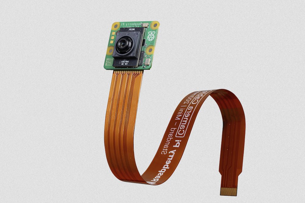
- Capture. The image sensor integrates light during the exposure time, then reads the pixels out, typically over a MIPI CSI-2 link. With a rolling shutter, different rows are exposed at different times, so “the timestamp of a frame” needs a precise definition.
- ISP. A hardware image signal processor turns raw Bayer data into a usable image. It handles demosaicing, noise reduction, white balance, tone mapping and often lens correction and scaling.
- Preprocessing. The frame is resized, cropped, color-converted and normalized into the tensor layout the model expects. This runs on the CPU, GPU, or a dedicated 2D engine.
- Inference. A neural network, or a classical vision algorithm, runs on an NPU, GPU, DSP or CPU.
- Post-processing. Decoding detections, non-maximum suppression (NMS), tracking across frames, and fusion with other sensors.
- Actuation or output. Issuing a command (stop the conveyor, steer, raise an alarm), or encoding and streaming metadata and video to an operator or server.
An illustrative latency budget
The table below is a hypothetical budget for a 30 fps detection system with a target end-to-end latency of about one frame period (33.3 ms). The numbers aren’t measurements of any product. They show how a budget is structured and where variability comes from.
| Stage | Typical hardware | Illustrative budget | Main sources of variability |
|---|---|---|---|
| Exposure + readout | Sensor, CSI-2 receiver | 12 ms | Auto-exposure changes, readout time, sensor mode |
| ISP | Hardware ISP | 3 ms | Resolution, HDR modes, memory contention |
| Preprocessing | CPU / GPU / 2D engine | 2 ms | Cache behavior, competing CPU load |
| Inference | NPU / GPU | 10 ms | Memory bandwidth, accelerator sharing, thermal throttling |
| Post-processing | CPU | 2 ms | Number of detections (NMS, tracking) |
| Decision + actuation | CPU / MCU, fieldbus | 3 ms | Bus arbitration, network latency |
| Total | 32 ms |
Deadlines, latency, throughput and jitter
Engineers often say “the system runs at 30 fps” as if that settled the timing question. It doesn’t. Three different requirements are involved:
- Throughput: the system must process frames at the camera rate, or at a defined fraction of it. Every stage’s average processing time must fit within the frame period.
- End-to-end latency: the time from the physical event, approximated by the start of exposure, to the resulting action. Control loops, safety interlocks and human-in-the-loop systems care about this.
- Jitter: variation in latency or in output timing. Trackers, controllers and video playback all degrade when inter-frame timing is irregular, even if the mean is fine.
Pipelining lets each stage work on a different frame at the same time. That raises throughput without changing per-frame latency, but queues between stages add waiting time. With three frames buffered between capture and inference, the result describes a scene that is already about 100 ms old at 30 fps. For actuation, the age of the data matters more than the frame rate.
Most vision deadlines are firm. A late result isn’t catastrophic, but it has no value, and processing it wastes resources that newer frames need. Our introduction to hard, firm and soft deadlines covers this classification. Firm deadlines suggest better metrics than the average: the deadline-miss ratio, the longest run of consecutive misses, and (m,k)-firm constraints, which require at least m of every k consecutive frames to meet their deadline.
Define your timestamps. On Linux, V4L2 buffers carry timestamps and flags that say whether the time refers to start of exposure or end of frame. Decide which reference your latency requirement uses, and propagate that timestamp through every stage. Otherwise you can’t measure end-to-end latency honestly.
Modeling the pipeline as real-time tasks
For analysis, treat each stage as a task in a cause-effect chain. Stages may be released by the camera’s frame interrupt (event-triggered) or run periodically and read the newest available data (time-triggered). The difference matters. Event-triggered chains have lower latency but propagate jitter. Time-triggered chains are easier to analyze but can add up to one period of sampling delay per stage boundary.
A robust pattern for firm deadlines is the latest-value mailbox. Each stage overwrites a single-slot buffer instead of appending to a queue, so downstream stages always see the freshest frame and stale frames are dropped automatically:
// Single-slot "latest frame" handoff with a latency check
on_frame_ready(buf):                 // camera / ISP completion
    mailbox.replace(buf)             // overwrite unprocessed older frame

inference_task():                    // e.g. a SCHED_DEADLINE thread
    loop:
        f   = mailbox.take_latest()  // blocks until a frame is available
        age = now() - f.t_exposure
        if age + WCET_INFER + WCET_POST > LATENCY_BUDGET:
            stats.dropped += 1       // cannot finish in time: skip it
            continue
        dets = npu_run(model, preprocess(f))
        publish(postprocess(dets), f.t_exposure)
On Linux, give each stage thread an explicit scheduling policy. SCHED_FIFO with carefully assigned priorities works, and SCHED_DEADLINE reservations isolate stages from one another and from best-effort load. Our article on SCHED_DEADLINE and the Constant Bandwidth Server explains how to size those reservations. Pin threads to isolated cores, steer camera and NPU interrupts away from them, and lock memory to avoid page faults. When a pipeline spans several cores, the partitioning trade-offs in multicore real-time scheduling apply directly.
Accelerators: NPUs, GPUs and DSPs
Accelerators make modern edge inference feasible, but they break several assumptions of classical scheduling theory.
Non-preemptive execution
Many NPUs and embedded GPUs run a submitted inference job, or at least each kernel or layer, to completion. A high-priority, low-latency model may then have to wait for a long, low-priority job that is already on the accelerator. That wait is a blocking term, just like a lower-priority critical section in priority inversion analysis. Its length is the longest non-preemptive segment of any lower-priority job. Splitting large models into smaller submissions shortens that blocking at the cost of more overhead.
Shared memory bandwidth
The ISP, NPU, GPU, display controller and CPU cores usually share one DRAM interface. A neural network that streams large weight tensors can slow the ISP or a CPU control task significantly. These interference effects don’t show up when you benchmark each component alone. Treat memory bandwidth as a shared resource. Measure stage timings under realistic concurrent load, and where the platform supports it, use bandwidth regulation or QoS settings.
Batching and runtime overheads
Batching several frames per inference improves accelerator efficiency but adds up to a full batch of waiting time per frame. It suits offline analytics, rarely real-time actuation. Also watch for one-time costs that can surprise you at run time: model loading, graph compilation, memory allocation and “first inference” warm-up. Do these at initialization, not on the first real frame.
Timing analysis for inference workloads
Static WCET analysis of a full DNN on a GPU or NPU is generally impractical with current tools. Accelerator microarchitectures are often undocumented, and memory interference dominates. That said, a conventional CNN’s control flow is largely data-independent. It performs the same layers and operations for every frame, so its execution time tends to be much more stable than that of general-purpose code. The variable parts are usually elsewhere:
- Post-processing scales with the number of candidate detections. NMS on a cluttered scene can take much longer than on an empty one, so bound the number of candidates.
- Dynamic networks with early exits, attention over variable-length inputs, or region-based stages have input-dependent cost.
- Contention and thermal state change accelerator throughput at run time.
In practice, teams use measurement-based timing analysis: long runs over representative and adversarial inputs, under worst-case concurrent load, at the lowest sustained clock frequency, with high-water marks and latency histograms recorded per stage. The limitations of this approach, and the hybrid methods that improve on it, are covered in WCET analysis methods. Add a margin and monitor deadlines at run time so the system can detect and react when assumptions are violated.
Thermal reality check. Accelerators that hit their benchmark latency on a cool bench may throttle after minutes of sustained load in an enclosure. Characterize timing at the steady-state temperature of the deployed product, not just at power-on. Energy and thermal behavior are discussed further in energy-aware real-time scheduling.
Graceful degradation and adaptive quality
Video workloads vary: scene complexity, detection counts and concurrent streams all change over time. Rather than provisioning for an extreme worst case that rarely happens, many systems define several quality levels and switch between them at run time:
- process every second or third frame (controlled frame skipping) instead of dropping frames at random;
- reduce input resolution, or process only regions of interest flagged by a cheap motion detector;
- switch to a smaller, faster model variant under load;
- lower the encoding bitrate or resolution of outgoing video before the analytics path is touched.
This is exactly the problem that contract-based and reservation-based scheduling address. Each component declares a minimum acceptable budget and can use more when spare capacity exists. The original FRESCOR research project chose video-centric applications as evaluation domains. Two of its three were a multimedia phone with video streaming and a digital video surveillance system; the third was software-defined radio. The project archive’s expected results page describes the goals, and contract-based scheduling explained shows how minimum and desired budgets map onto quality levels.
Separate the critical path. If a vision system drives a safety-relevant actuator, keep the safety decision on a small, analyzable path, such as a dedicated MCU or a high-priority reservation. Keep best-effort analytics and streaming isolated from it. The design patterns in mixed-criticality systems apply directly. For networked cameras, see real-time networking with TSN for transport guarantees.
Before committing to hardware, it helps to model the pipeline’s stage budgets as a task set and check feasibility. Our schedulability calculator handles the CPU-side tasks. For a full end-to-end review covering accelerators and memory contention, see our schedulability audit.
Frequently asked questions
What frame deadline should I use for a 30 fps camera?
The frame period (33.3 ms) is the throughput constraint: each stage must keep up on average. The latency deadline comes from the application, such as how quickly a robot must stop. It may be shorter or longer than one frame period. Specify both separately.
Should I queue frames or drop them when the system falls behind?
For actuation and alarms, drop stale frames and process the newest one, because a queue only adds latency. For recording or offline analytics, where every frame matters and latency doesn’t, queuing is appropriate.
Can an NPU be preempted by a higher-priority model?
It depends on the hardware and driver. Many accelerators only switch between jobs at job or layer boundaries. Treat the longest non-preemptive segment of lower-priority work as a blocking term, and check the vendor documentation for priority or preemption support.
Is average inference latency a useful metric?
Only for capacity planning. For real-time behavior, look at the latency distribution’s tail (high percentiles and observed maximum) under worst-case concurrent load, along with deadline-miss ratio and consecutive misses.
Does a global shutter sensor improve timing?
It gives every pixel the same exposure interval, which removes rolling-shutter skew and makes the frame timestamp unambiguous. It doesn’t remove readout or processing latency.
References and further reading
- Video for Linux API (V4L2) — Linux kernel documentation
- Deadline Task Scheduling — Linux kernel documentation
- Image processor — Wikipedia
- Camera Serial Interface (MIPI CSI) — Wikipedia
- Rolling shutter — Wikipedia
- AI accelerator — Wikipedia
- FRESCOR — Framework for Real-time Embedded Systems based on COntRacts, EU FP6 project IST-034026 (2006–2009), project record on CORDIS.